Dirichlet Process for mixture modeling and Application

Introduction

Parametric model suffer over-under fitting and are subject to model selection. The bayesian nonparametric framework offer an alternative with a model complexity that adapts to the number of data in an automatic and scientifically founded manner.

Assuming we have infinite, exchangeable data \(y_{1}, y_{2}, ...\) De Finetti’s theorem ensures the existence of a distribution \(G\) such that the predictive distribution is given by \(p(y_{1}, ..., y_{n}) = \int_{\Omega} p(y_{1}, ..., y_{n} | \theta)dG(\theta)\)

How can we know \(G\) ? The main idea is to consider \(G\) as a parameter to infer that lives in a space of distributions that put probability mass on sets \(A \subset \Omega\) . Bayesian inference then requires to elicitate a prior on \(G\) and allows us to define quantities such as \(E(G(A))\), \(Var(G(A))\) or \(G(A)|y_{1}, ..., y_{n}\).

With a specified observation model \(p(\theta | y)\) the posterior becomes \(p(\theta | y) \propto p(y|\theta)\int_{\mathcal{G}}p(\theta | G)\pi(dG)\)

Prior elicitation and careful modeling of the observation process still matter. The specified nonparametric model will have some structure that won’t adapt to every form of model mispecification.

Here we will review one nonparametric model, the Dirichlet Process, and implement it in the case of clustering.

The Dirichlet process

Formal Definition

The Dirichlet process is a stochastic process whose sample paths are probability measures. Given a distribution \(H\) and a positive parameter \(\alpha\), we have, for any finite partition \(A_{1}, ..., A_{n}\) of \(\Omega\):

We have \(E(G(A)) = H(A)\) and \(V(G(A)) = \frac{G(A)(1 - G(A))}{\alpha + 1}\).

Hence, \(H\) can be interpreted as the centered distribution and \(\alpha\) the precision towards the centered distribution. This define the prior distribution for our nonparametric model.

\(\theta_{i} \sim G\) are i.i.d, however, marginalized over \(G\) they are not independant, in particular, we can show that :

And, marginalized over \(G\):

These equations gives insight into a nex representation of the parameters that we will explore now.

The Chinese Restaurant process

As the previous equations show, we don’t expect all the \(\theta_{i}\) to have distinct values, we can thus reinterpret our parameters \((\theta_{i})_{i = 1:n}\) to the parameters \(\{ (\theta_{i}^{*})_{i = 1:K}, (S_{i})_{i = 1:K}\}\) where \(\theta_{i}^{*} \sim H\) and \((S_{1}, ..., S_{K})\) is a partition of \([n]\), where \(S_{k}\) corresponds to the labels \(i\) such that \(\theta_{i} = \theta_{k}^{*}\). From this interpretation, we can reformulate our previous equation to:

This operation is called the “Chinese restaurant process”, where the \((\theta_{i})_{i}\) can be interpreted as clients entering a restaurant, and choosing a table with a probability proportional to the number of clients sitting at this table, and a probability to choose a new table proportional to \(\alpha\).

By following this iterative process we can directly infer the joint probability of the reparametrization:

Where \(P_{\alpha}(S) = \frac{\Gamma(\alpha) \alpha^{K} \prod\limits_{k = 1}^{K}\Gamma(n_{k})}{\Gamma(\alpha + n)}\) can be directly inferred by developping the chinese restaurant process and rearranging the terms.

Stick Breaking Process

There exist a way to sample a distribution \(G\) from \(DP(\alpha, H)\) called the “stick breaking process” that works as follows:

• Sample \((w_{i})_{i = 1,...} \sim Beta(1,\alpha)\)
• Sample \((\theta_{i}^{*})_{i = 1,...} \sim H\)
• Compute \(\pi_{i}(w) = w_{i}*\prod\limits_{j = 1}^{i - 1}(1 - w_{j})\)
• Return \(G = \sum\limits_{i = 1}^{\infty} \pi_{i}(w)\delta_{\theta_{i}^{*}}\)

This interpretation is very insteresting, because we see that sampling a distribution according to the Dirichlet Process compute an infinite probabitily vector corresponding to parameters sampled from the base distribution \(H\).

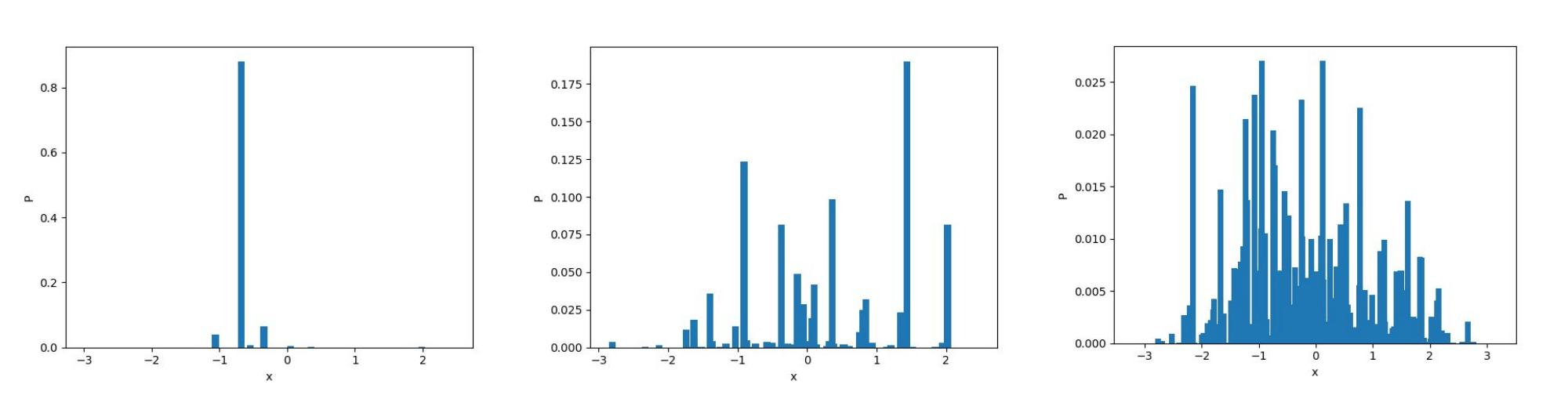
The code to reproduce this process can be found here.

Dirichlet process for Mixture

Finite Mixture Model

A finite mixture model assumes that the data come from a mixture of a finite number of distributions.

Here \(\pi\) are latent variables describing the cluster the data come from. \(H\) is the distribution the parameters of the observation model come from.

Dirichlet Process for Mixture

It can be showed that the marginal distribution of \(\theta_{i}\) in the finite mixture model converges in distribution to the marginal distribution of the Dirichlet Process for mixture modeling defined by:

Inference

In a DP model for mixture, we assume that the data are generated in the following way:

With the following prior for \(\theta\):

Hence, the Bayes rule translates into, with the representation given above:

The main techniques explored in order to perform inference are MCMC methods and Variational Inference methods. However, choosing the observation distribution \(f(y|\theta)\) to be conjugate with \(H\) allows us to design a Gibbs Sampler that greatly improve performances.

Gibbs Sampling

A Gibbs Sampler can be designed in the following manner to sample from the full posterior distribution \(p(\theta^{*},S | y )\):

If a new cluster is created, draw

Conjugate priors

In the case we model our observation \(y_{i} | \theta_{k}^{*}\) from a multivariate gaussian:

Then a conjugate prior for this distribution is the Normal-Inverse Wishart distribution with the four hyperparameters \((\boldsymbol{\mu}_{0}, \lambda, \boldsymbol{\Psi}, \nu)\):

In this case the posterior distribution can be written:

Where :

The predictive likelihood follows a multivariate student t distribution with \((\nu_{n} - d + 1)\) degrees of freedom that we will approximate by moment matching by a gaussian, which is a faithful representation (according to the Kullback-Leibler divergence) when \(\nu\) increases:

Simulation

The source code for the simulations can be found here. The Gibbs Sampler with the previous priors is implemented and supports data of any dimension.

from objectDP import DirichletMixtureConjugate
diri = DirichletMixtureConjugate(data)
diri.fit(epoch = 30, vis = True)

Dirichlet Process with 120 2D Gaussian points

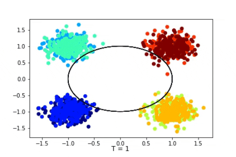
Dirichlet Process with 1600 2D Gaussian points

Dirichlet Process with 4000 2D Gaussian points

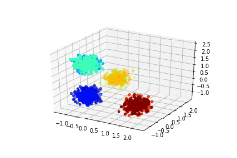
Dirichlet Process with 1600 2D Gaussian points

We can see that in these cases the state of the sampler quickly attain the expected states and stay in them consistently. Of course, in a Bayesian setting, we should, instead of displaying the state of the Markov Chain, study the posterior distribution of certain quantity of interests such as the number of clusters, and then infer chosen estimators, such as the mode of the posterior mean. Here we suppose that the states quickly attain the mode of the posterior.

Discussion

This model allows to perform non parametric bayesian inference, however, it shifts the problem to the design of the prior which establish the size a priori of a cluster. It is interesting to note that one particular modification of the Dirichlet Process, calles the Pitman-Yor process has attracted attention, especially because it gives a power-law like distribution over the parameters (the infinite probability vector we talked about), and thus gives more flexibility for modelling certain type of data with the same behaviour.

Note on model extension.

Taking one additional step of abstraction: The Hierarchical Dirichlet Process

Imagine the data comes from different groups. For instance, in the problem of Topic Modelling, which consists in discovering the abstract “topics” that occur in a collection of documents, one can model a document as a mixture of latent topics, and each topic as a mixture of words. In this model (described by the Latent Dirichlet Allocation), the model has a Hierarchical structure, ie, the distribution of words in a document is conditioned by the distribution of the document over topics the word belongs to. Certain Hierarchical structure, whose hierarchy can be arbitrarily extended and represented in a tree structure, can be naturally modeled by Hierarchical statistical model, such as the Hierarchical Dirichlet Process among others, described as follows:

Here, \(J\) represents the number of groups (the documents in the case of topic modelling). Whithin this group, the configuration is the same as a classic Dirichlet Process:

Where \(F\) is the observation model. In this model, an extension of Chinese Restaurant Process and the Stick Breaking Process exist to treat this configuration. One can see the original paper for more details.